On heterozygosity at a locus under selection
February 5, 2025
Pairwise heterozygosity – or the probability that two alleles sampled from a population differ at a locus – is a measure of genetic diversity widely employed in population genetics. Mathematically, it can be expressed as
$ \displaystyle{H = \langle 1 - \sum_i f_i^2 \rangle} $,
where $f_i$ denotes the population frequency of allele $i$, and the expectation $\langle .\rangle$ is taken over independent realizations of evolutionary dynamics.
In the simplest model of evolution, $f_i$ depends on the rate at which loci mutate between allelic states, selection acting on fitness differences conferred by mutation, and random drift arising due to finite population size $N$. For $i\in\{0,1\}$, corresponding to the one-locus two-allele haploid1 model, a solution for the allele frequency distribution was first derived by Wright (1937) in the limit of large $N$. Moments such as $H$ can be straightforwardly calculated from this distribution.
We forgo the aforementioned result and instead propose a heuristic argument2. If mutation is infrequent (such that $0\rightarrow1$ flips occur at a total rate $N\mu \ll 1$ per unit time), the population comprises primarily wildtype alleles. The vast majority of mutant lineages are short-lived, vanishing after only a few generations due to drift. However, some will survive long enough to reach appreciable frequencies. These dynamics are transient: eventually, each mutant lineage will either go extinct or take over the population3. The details of this process depend strongly on how mutation affects fitness.

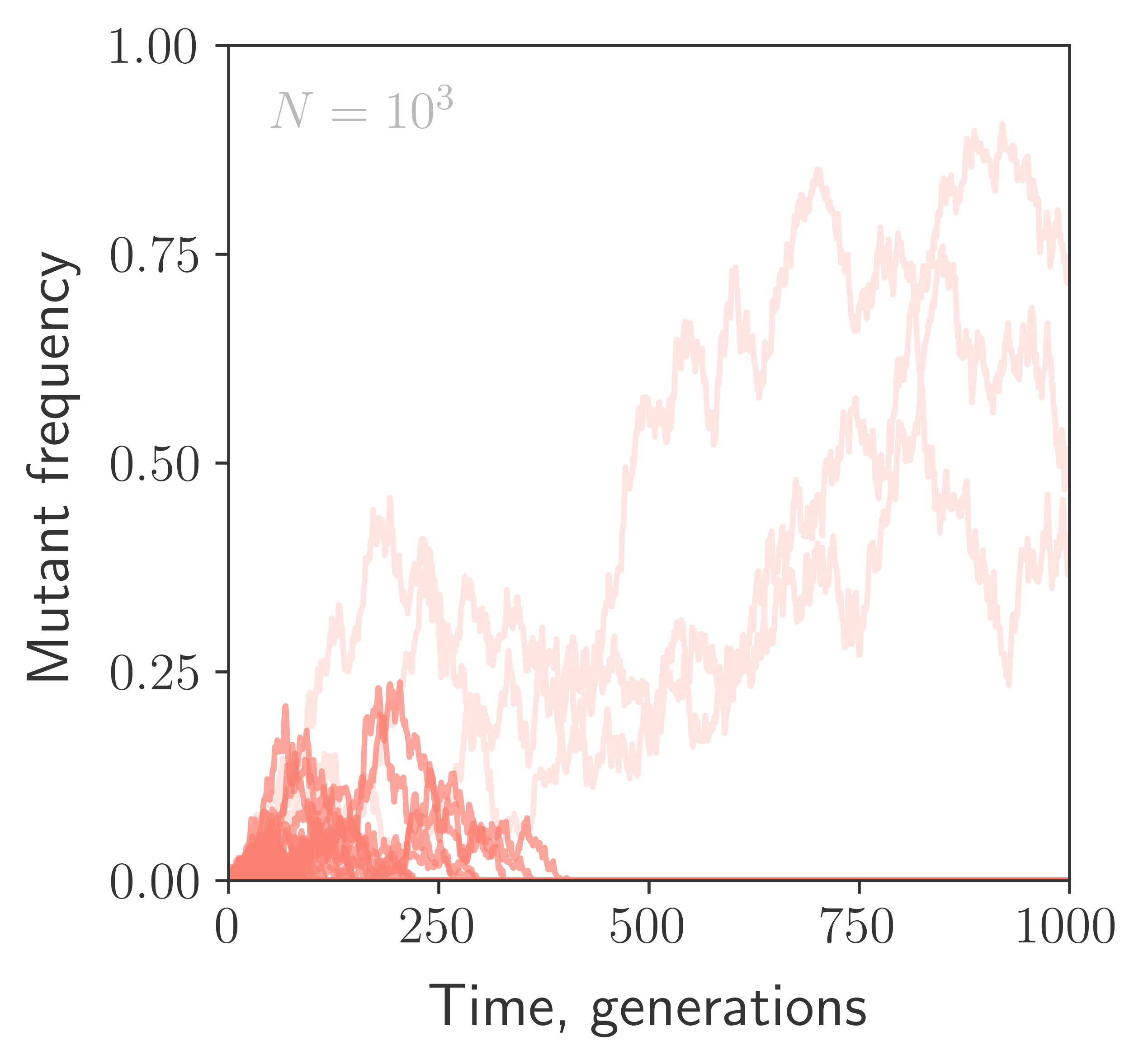
One thousand simulated mutant trajectories in a population of size $N=10^3$, with the mutation having no impact on fitness. Extinct trajectories are highlighted.
Neutral alleles
If mutation has no effect on fitness, the frequency of a mutant lineage is only influenced by drift. With probability $1/t$, this lineage will survive for at least $t$ generations, reaching a characteristic size of $f \sim t/N$. A more rigorous calculation (Kendall, 1948) shows that the frequency of the surviving lineage is exponentially distributed around this characteristic size,
$ \displaystyle{p(f|f>0) df \sim \frac{N}{t} e^{-Nf/t} df} $,
which implies that, on a logarithmic scale, most of the probability density is contained within $\sim \mathcal{O}(1)$ of $\log (t/N) $.
The allele frequency distribution can be understood in terms of the number of mutant lineages that end up in the frequency range $\log f \pm \mathcal{O}(1)$ at time $t$. The rate at which mutant lineages reach frequency $f$ is $N\mu \cdot 1/Nf$, and lineages that do so must have originated within $\Delta t \sim Nf$ generations in the past. Summing up their contributions yields
$ \displaystyle{p(\log f) \sim N\mu \cdot \frac{1}{Nf} \cdot \Delta t \sim N\mu} $,
emphasizing that $p(f)$ is evenly distributed on a logarithmic scale, with equal contributions from all orders of magnitude in $f$. Switching back to a linear scale, we recover the familiar allele frequency distribution,
$ \displaystyle{p(f) \sim \frac{N\mu}{f}}$.
Note that this calculation is only valid for $t \ll N$. At longer times, there is $\sim\mathcal{O}(1)$ probability that a mutant lineage will have reached $f\sim 1$, or fixed. For a steady state to exist, we thus need an influx of new mutations; Ewens (1963) showed that this can be achieved by restarting the process at some infinitesimal frequency $\epsilon$ immediately upon fixation4.
The pairwise heterozygosity is therefore given by
$ \displaystyle{H \sim \langle f(1-f) \rangle \sim \int_{\epsilon}^1 f(1-f) p(f) df \sim N\mu} $,
in agreement with the exact result $H=2N\mu$ up to an $\sim\mathcal{O}(1)$ constant.
Deleterious alleles
The frequency dynamics of alleles with a fitness cost $s$ differ only in that selection prevents them from reaching frequencies much larger than $1/Ns$, preserving the shape of $p(f)$ below $f\sim 1/Ns$. We can see that moments of the frequency distribution such as $H$ will be dominated by these frequencies, provided $Ns \gg 1$,
$ \displaystyle{H \sim \int_{0}^{1/Ns} f(1-f) p(f) df \sim \frac{\mu}{s}}$.
Beneficial alleles
Just like deleterious alleles, strongly advantageous alleles with fitness benefit $s$ will remain invisible to selection at frequencies below $1/Ns$. However, if they drift to this frequency, they begin to expand deterministically due to selection as
$ \displaystyle{\partial_t f = sf(1-f)}$.
As they sweep through the population, they will contribute to heterozygosity
$ \displaystyle{H \sim N\mu \cdot s \cdot \int_{0}^{1/s \log Ns} f(1-f) dt \sim N\mu \cdot s \cdot \frac{1}{s} \sim N\mu} $,
which is much larger than the contribution from lineages that are still drifting since $Ns \gg 1$. Therefore, perhaps surprisingly, we see that beneficial mutations give rise to heterozygosity similar to that observed for neutral mutations. This is because while beneficial alleles reach frequencies where $f(1-f) \sim \mathcal{O}(1)$ with probability $s$, they spend only $1/s$ generations passing through.
Thanks to Maike Morrison for encouraging me to think this through, and to Zhiru Liu and James Ferrare for helpful discussions.
1 In diploid organisms, heterozygosity often refers to the probability that two alleles at a locus differ in state within an individual, rather than across the population. If the dominance coefficient is $1/2$, the diploid system is equivalent to the haploid case considered here, with a rescaled population size. Other kinds of dominance fall outside our simple model.
2 This argument follows from the work of Desai and Fisher (2007), Weissman et al. (2009), Cvijović et al. (2018), and Good (2022).
3 Note that at long times, it is sufficient to know the probability mass at $f_i = 1$, or the fixation probability, to find the first moment of the distribution. This is not the case for higher moments, which depend on the lineage trajectory in addition to its ultimate fate. This distinction between divergence statistics such as $\langle f_i \rangle$ and polymorphism statistics such as $\langle f_i^2 \rangle$ underlies many inference approaches in population genetics (see e.g. McDonald and Kreitman, 1991).
4 Specifically, reinstating the mutant lineage in this way changes the overall normalization constant of the distribution $p(f)$, but does not alter its shape.